Excel spreadsheets support lookup functions that return a value from a table by looking up another value in the table. The vlookup and hlookup functions in Excel work as one-way lookups. This article helps you to perform a two way lookup.
The Pi
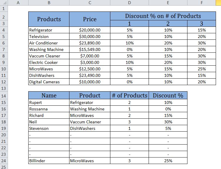
cture below shows a simple example:

The first table shows products, Price of the product and discount on number of products purchased. The second table shows name of the person, product purchased, number of products purchased and discount applicable.
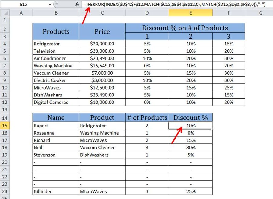
A formula is used in column E of second table to get the discount percentage from the first table as shown in the picture below:

The formula in cell E15 looks up the values of cells C15(Product) and D15(# of Products) in the first table and returns the corresponding value from the table.
The formula in E15 is:
=IFERROR(INDEX($D$4:$F$12,MATCH($C15,$B$4:$B$12,0),MATCH($D15,$D$3:$F$3,0)),”-“)
Description of the formula:
The above formula uses the INDEX function, which consists of three arguments.
 The first argument gives the entire range of ‘Discount% on # of products’ from first table($D$4:$F$12).
=IFERROR(INDEX($D$4:$F$12,MATCH($C15,$B$4:$B$12,0),MATCH($D15,$D$3:$F$3,0)),”-“)
 The second argument is MATCH function. MATCH ($C15,$B$4:$B$12,0)
It matches the ‘product’ in cell C15 of second
table with the ‘products’ in cells B4 to B12 of first table and returns the ‘Product‘.
=IFERROR(INDEX($D$4:$F$12,MATCH($C15,$B$4:$B$12,0),MATCH($D15,$D$3:$F$3,0)),”-“)
 The third argument is also a MATCH function. MATCH ($D15,$D$3:$F$3,0).
It matches the ‘# of products’ in cell D15 of second table with the ‘Discount% on # of products’
in cells D3 to F3 of first table and returns the ‘# of products’.
=IFERROR(INDEX($D$4:$F$12,MATCH($C15,$B$4:$B$12,0),MATCH($D15,$D$3:$F$3,0)),”-“).
In this way the above formula is used as a two way lookup formula to retrieve the value required.

