November 2019 - Your Excel Partners

November 28, 2019January 9, 2020

How to accelerate excel performance?

Efficiency is one of the key elements to evaluate any application. Excel has always topped the race in efficiency when compared to other spreadsheet applications. But there are some instances where Excel lags in performance which could affect productivity. In this article let us look at some of the key elements that would help to enhance the performance of Excel.

Excel 2007 and later versions have “Big grid” (1 Million rows and 16,000+ columns) compared to their previous versions. Since the capacity of the application has increased, there are more chances for performance degradation as we would be dealing with huge amount of data.

1. Switch to Manual Calculation mode from Automatic

By default, automatic calculation is the default option while working on Excel. In this mode, whenever we change the content of any cell in our workbook, all formula in all cells of all open workbooks would be recalculated. We won’t realize the time spent in formula recalculation as long as it is less than a tenth of a second, all put together. As this calculation time increases, annoyance starts to increase, especially for repetitive tasks. In this situation’s users can switch to “Manual calculation” option in the formulas tab. In this mode, formula would be recalculated only when ‘Calculate Now’ or ‘Calculate Sheet’ button is pressed.

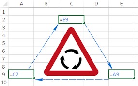
2. Avoid Circular references

As calculations are single threaded, multiple references to one or more formula could slow down the performance. Minimizing the use of circular references can boost the formula calculation time.

3. Avoid links across workbooks

Try to avoid links between workbooks. If links are not removed, opening of that workbook could end up in evaluating the link from the source. This can easily increase the calculation time. Best practice is to paste special the formulas into values, which can save your memory and increase calculation time as well.

4. Write efficient formulas

Writing efficient formulas will add value to the calculation time. Nested formulas, array formulas, unsorted columns, redundant data can lead to performance degradation. For example, VLOOKUP and HLOOKUP with exact match would take more calculation time than approximate match after sorting the same data. So, better understanding of logic and using the right formula can increase Excel performance.

5. Use conditional formatting cautiously

We should be very cautious while using any formatting option in Excel, especially while using conditional formatting because of its volatile nature. Apply the formatting only to the used range and make sure you haven’t selected the entire column/row while applying these formats. This can increase Excel performance.

There are many other elements to be considered to improve performance of an application. The above mentioned are few among them and these are the key to accelerate the performance of an Excel application.

Check out our Tableau pages

November 25, 2019November 19, 2019

Intro to Power query in Excel

This tool is generally referred to as ‘Power Query’ when searching for information online. However, with Excel 2016, the tool is also commonly referred to as ‘Get and Transform’. It can link to external data from many different types of sources into local data model in Excel or display them as tables. It uses the M Language to record each step we make and lets us to modify those steps in way we want.

Power Query is one of the most powerful tools added to Excel. There is lot of potential to save time in repetitive data cleaning and formatting using this. It can be accessed by clicking Data -> Get Data -> Launch Power Query editor.

Connect, Transform, Combine and Share are the sequence of steps to blend data make the data model, using Power Query.

Connect

Power Query can be connected to single or multiple data sources like Excel workbook, databases, feeds and cloud services. Microsoft always updates the new data connections to Power Query, so you should update the App to get them added.

Once you connect to any of the data sources then you can directly load data into excel or edit using Power Query by clicking on the option provided. The below snap shows the number of data connections available in Power Query.

Transform

Power Query lets you remove column, change data type, merge tables etc. Each of these actions is a transformation. The above-mentioned options are available in Query Editor/Transform of the Power Query ribbon. The Query Editor records each step you apply to the data.

Combine

You can combine data from multiple data sources into single data model to get unique view into the data. There is no specific option called combine in Power Query. You can achieve this by writing a query or merge/grouping different tables and make them a single table with a unique reference. We can load the merged data into excel for further analysis.

Share

After applying all the conditions/queries on the loaded data. The result will be the processed information. We can save, share or use it for further analysis. Typically, you can use these reports in excel, power BI or any other BI tools for analysis and visualization.

November 21, 2019January 9, 2020

MS Excel and ODBC/OLEDB for Database connectivity

Flat files like Excel workbooks have limitations when it comes to data storage. Though the new release of Excel has enough number of rows and columns to accommodate and analyze data, working with huge flat files in an Excel is a difficult job. Here comes the ‘database’, for our rescue.

A relational database management system (RDBMS) is an organized way of storing huge amounts of structured/columnar data. It also allows us to access the required records through SQL queries (SQL – Structured Query Language). MS Access, MS SQL server, Oracle, DB2 etc. are a few popular RDBMS.

This article is all about connecting Excel to MS Access & SQL Server using ODBC or OLEDB connection string. ODBC or OLEDB are the mediums to connect databases to any application.

Connecting to MS Access from Excel (2016)

The below procedure uses OLEDB connection string to establish the connection between the applications. To import data into an Excel workbook from MS access, there should be at least one table inside MS Access database. Save the created database in any location.

Step1: Open Excel Application -> Data tab -> Get Data -> From Database -> From MS Access Database.

Step2: Then select the database file located on your drive and then double click the “Table” you want to import.

Step3: You will get an option to edit the table in a “Power Query” editor as shown below.

Step4: Click on “Click & Load to” option on the top left section of the ribbon. Then you will get a pop up to select the destination cell as shown below.

Step5: Click ‘OK’ to get the data into the selected range of the excel worksheet. The data is dynamic, once MS Access table gets updated, same can be reflected into Excel workbook by clicking “Refresh All” option in the “Data Tab“.

Connecting to SQL Server Database from Excel

Connecting SQL has same type of data connectivity as MS Access, but the only difference is to enter the SQL server name in the field provided. Please refer below image.

Open Excel -> Data Tab -> Get Data -> From Database -> From SQL Server Database -> Enter SQL server name -> Enter Login Credentials -> click Next -> Select the database and table -> Click Next -> Select the cell/range to load the SQL table content -> Click OK

Connecting any database from Excel application follows the above procedure in establishing the connection. We can also use Visual Basic programming to automatically connect and refresh data from the database.

Check out our Tableau Pages

November 19, 2019January 9, 2020

How to create multiple dependent drop-downs using array formulas in Excel?

Drop-down lists are a very important part of any dashboard or data entry form. In this article, we’ll learn how to create multiple dependent drop-downs using array formulas. What I mean by multiple dependent drop-downs is: When selecting an item from the first drop-down, the following drop-downs would show only relevant items based on your selection.

Creating dependent drop-down lists in excel could be easy if done using VBA, but it becomes trickier to do it with excel formulas alone. For this, we can use ‘Array formulas’. An array is a collection of one or more items. Likewise, an array formula can return one or more items as result. Array formulas must be entered in a cell by pressing Ctrl + Shift + Enter. In the formula bar, you can see any array formula wrapped inside curly braces {}. For example, {SUM(A1:A5)}

We have sample data as follows:

Using the above data, we want to create dependent drop-downs like shown below. To create these drop-down lists, I will be using two sheets: “Sample Data” & “Temp”.

Creating a list with unique values for first drop-down

In Column A of ‘Sample Data’ , you can see there are repeated values. We need to eliminate them before we can show it in our first drop-down . There are many ways to make a list unique. One option that is often used is ‘Remove duplicates’ feature from ‘Data’ tab of Excel’s menu ribbon. But using that is a manual task and must be repeated, when new data would be added. Hence, it is not preferred. Another option to get the unique list would be to use array formulas. The below formula can be used to get the unique values from column A of ‘Sample Data’.

Write the below formula in the “A2” cell of “Temp” sheet and remember to press Ctrl + Shift + Enter! Drag the formula till “A11” cell of “Temp” sheet.

IFERROR( INDEX( SampleData!$A$3:$A$11,MATCH( 0, COUNTIF( $A$1:A1,SampleData!$A$3:$A$11), 0) ) ,””)

COUNTIF function would return the number of occurrences of the in the sample data range
MATCH function will look-up for”0” in the output of COUNTIF and returns the row number which has the next unique brand name
INDEX function picks up & shows the text of the next unique brand name from the respective row number given by MATCH
If MATCH does find anymore unique names on the sample data range, then it’ll return #N/A error instead of row number, which would be handled by IFERROR function

Thus, unique list of values for column A of Sample Data would be obtained in “Temp” sheet.

First dynamic range drop-down

To populate the obtained unique values into a drop-down list, we’d use the data validation feature from ‘Data’ tab of Excel’s menu ribbon. Since we don’t know how many unique brand names could be there at any point in time, we cannot use a fixed range to populate the drop-down. We must use a dynamic range to populate the drop-down list.

In cell “A16” of “Sample Data” sheet, write the below formula in the Data Validation window and click OK as shown in the below Figure to get the dynamic drop-down list as shown below.

OFFSET(Temp!$A$2,,,COUNTIF(Temp!$A$2:$A$30,”?*”),)

COUNTIF function would return the number of rows with brand names
OFFSET function would select the number of rows as given by COUNTIF from A2 and populate the dynamic drop-down list

Second dependent dynamic range drop-down

Creating the second drop-down involves the same task as we did before. But, the second drop-down should populated on selecting an item from the first drop-down list. Thus, it should check the selected item in the first drop-down (currently in “A16” cell of “Sample Data” sheet) an get only the relevant items. We achieve that by using the “IF” function.

Compared to the previous formula, the change in this array formula is the input array for the INDEX function. In previous formulas, the input was fixed to SampleData!$A$3:$A$11 . Here, the input array in which the unique values must be found should be based on the selection made on the previous drop-down and hence, is dynamically obtained using OFFSET formula.

Write the below formula in cell “B2” of “Temp” sheet, press Ctrl+Shift+Enter & drag the formula till “B11”.

IFERROR(

INDEX(OFFSET(SampleData!$B$2,MATCH(SampleData!$A$16,SampleData!$A$3:$A$11,0),0,COUNTIF(SampleData!$A$3:$A$11,SampleData!$A$16),1),

IF(AND( ISERROR( MATCH( 0, COUNTIF( $B$1:B1, OFFSET( SampleData!$B$2, MATCH( SampleData!$A$16, SampleData!$A$3:$A$11, 0), 0, COUNTIF( SampleData!$A$3:$A$11, SampleData!$A$16), 1) ), 0) )=TRUE, $B1=”HeaderName”), 1,MATCH(0,COUNTIF($B$1:B1, OFFSET( SampleData!$B$2, MATCH( SampleData!$A$16, SampleData!$A$3:$A$11, 0), 0, COUNTIF( SampleData!$A$3:$A$11, SampleData!$A$16), 1) ), 0) )),””)

In Cell “B16” of “Sample Data” sheet, using data validation, enter the below formula and click OK to get the dependent dynamic second drop-down list. Eventually, the output would look as shown below.

OFFSET(Temp!$B$2,,,COUNTIF(Temp!$B$2:$B$30,”?*”),)

Creating dependent drop-down using data validation and array formulas

Multiple dependent dynamic range drop-downs

Any number of further dependent drop-downs we create would follow the same procedure, but for more than two drop-down selections, the above formulas would become very long & difficult to handle. Instead of IF condition, we can use logical AND concept to get the same output. So, we can use the below formula from third drop-down to all further ones.

Write the below formula in cell “C2” of “Temp” sheet to get the unique values for third drop-down.

IFERROR(INDEX(SampleData!$C$3:$C$11,AGGREGATE(15,3,((SampleData!$A$16=SampleData!$A$3:$A$11)* (SampleData!$B$16=SampleData!$B$3:$B$11))/((SampleData!$A$16=SampleData!$A$3:$A$11)* (SampleData!$B$16=SampleData!$B$3:$B$11))*(ROW(SampleData!$B$3:$B$11) – ROW(SampleData!$B$2)), ROWS($B$1:$B1))),””)

AGGREGATE function is used here to get the smallest number in the range. The * operator performs logic AND operation.

In Cell “C16” of “Sample Data” sheet, using data validation, enter the below formula and click OK to get the dependent dynamic third drop-down list.

OFFSET(Temp!$C$2,,,COUNTIF(Temp!$C$2:$C$30,”?*”),)

The final output after we repeat the process for fourth and fifth drop-downs, would look as shown in the below Figure.

Conclusion

Creating drop-down with array formulas is fun. I hope this article would help you in creating more sophisticated dashboards with multiple dependent dynamic drop-downs.