The wait is over!! Finally, Microsoft has released an update to Office365 with a brand-new formula “XLOOKUP”.
XLOOKUP has the following advantages, compared to its predecessors.
- Can lookup on both left and right directions.
- Exact match is default.
- Can return FIRST or LAST match.
- XLOOKUP also replaces VLOOKUP & HLOOKUP.
Earlier, INDEX-MATCH formula combination was used to lookup values where HLOOKUP & VLOOKUP fell short. Now, XLOOKUP can replace all other functions. It is a robust and easy to use formula which can lookup values from right to left and vice versa.
Syntax:
=XLOOKUP(lookup_value,lookup_array,return_array,[match_mode],[search_mode])
Explanation
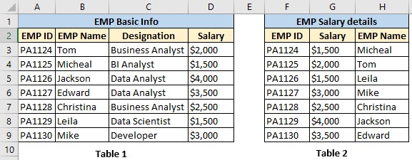
Let us consider the below example to get deep insight of the formula. Our agenda is to fill column D of Table1 (Salary) using XLOOKUP
Lookup_value: Exactly same as VLOOKUP. In this scenario, let us consider Column B of Table1 as our lookup value.
Lookup_Array: Typically, the destination range/column where XLOOKUP will look for the match. Column H of Table2 would be our lookup array.
Return_Array: This argument is asking for the return value. In this case, we want salary column to be filled so we would consider Column G of Table2 as the return value.
[match_mode]: This is an optional argument in XLOOKUP formula. It can be any one of the following. By default, it is “Exact Match”.
- 0 – Exact match
- -1 – Exact match or next smaller item
- 1 – Exact match or next larger item
- 2 – Wildcard character match.
[Search_mode]: It can be either 1 or -1. “1” is to search from first to last and “-1” is from last to first.
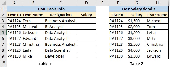
Let us write the below formula in cell “D3” of table1 and the output looks as below.
XLOOKUP($B$3:$B$9,$H$3:$H$9,$G$3:$G$9,0,1)