Drop-down lists are a very important part of any dashboard or data entry form. In this article, we’ll learn how to create multiple dependent drop-downs using array formulas. What I mean by multiple dependent drop-downs is: When selecting an item from the first drop-down, the following drop-downs would show only relevant items based on your selection.
Creating dependent drop-down lists in excel could be easy if done using VBA, but it becomes trickier to do it with excel formulas alone. For this, we can use ‘Array formulas’. An array is a collection of one or more items. Likewise, an array formula can return one or more items as result. Array formulas must be entered in a cell by pressing Ctrl + Shift + Enter. In the formula bar, you can see any array formula wrapped inside curly braces {}. For example, {SUM(A1:A5)}
We have sample data as follows:
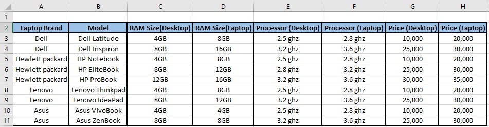
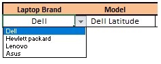
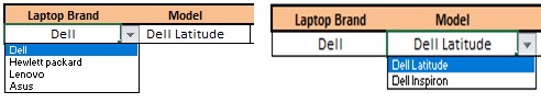
Using the above data, we want to create dependent drop-downs like shown below. To create these drop-down lists, I will be using two sheets: “Sample Data” & “Temp”.

Creating a list with unique values for first drop-down
In Column A of ‘Sample Data’ , you can see there are repeated values. We need to eliminate them before we can show it in our first drop-down . There are many ways to make a list unique. One option that is often used is ‘Remove duplicates’ feature from ‘Data’ tab of Excel’s menu ribbon. But using that is a manual task and must be repeated, when new data would be added. Hence, it is not preferred. Another option to get the unique list would be to use array formulas. The below formula can be used to get the unique values from column A of ‘Sample Data’.
Write the below formula in the “A2” cell of “Temp” sheet and remember to press Ctrl + Shift + Enter! Drag the formula till “A11” cell of “Temp” sheet.
IFERROR( INDEX( SampleData!$A$3:$A$11,MATCH( 0, COUNTIF( $A$1:A1,SampleData!$A$3:$A$11), 0) ) ,””)
- COUNTIF function would return the number of occurrences of the in the sample data range
- MATCH function will look-up for”0” in the output of COUNTIF and returns the row number which has the next unique brand name
- INDEX function picks up & shows the text of the next unique brand name from the respective row number given by MATCH
- If MATCH does find anymore unique names on the sample data range, then it’ll return #N/A error instead of row number, which would be handled by IFERROR function
Thus, unique list of values for column A of Sample Data would be obtained in “Temp” sheet.
First dynamic range drop-down
To populate the obtained unique values into a drop-down list, we’d use the data validation feature from ‘Data’ tab of Excel’s menu ribbon. Since we don’t know how many unique brand names could be there at any point in time, we cannot use a fixed range to populate the drop-down. We must use a dynamic range to populate the drop-down list.
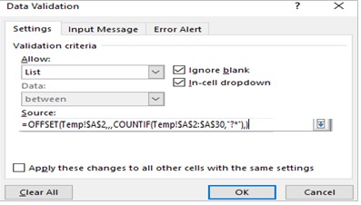
In cell “A16” of “Sample Data” sheet, write the below formula in the Data Validation window and click OK as shown in the below Figure to get the dynamic drop-down list as shown below.
OFFSET(Temp!$A$2,,,COUNTIF(Temp!$A$2:$A$30,”?*”),)
- COUNTIF function would return the number of rows with brand names
- OFFSET function would select the number of rows as given by COUNTIF from A2 and populate the dynamic drop-down list
Second dependent dynamic range drop-down
Creating the second drop-down involves the same task as we did before. But, the second drop-down should populated on selecting an item from the first drop-down list. Thus, it should check the selected item in the first drop-down (currently in “A16” cell of “Sample Data” sheet) an get only the relevant items. We achieve that by using the “IF” function.
Compared to the previous formula, the change in this array formula is the input array for the INDEX function. In previous formulas, the input was fixed to SampleData!$A$3:$A$11 . Here, the input array in which the unique values must be found should be based on the selection made on the previous drop-down and hence, is dynamically obtained using OFFSET formula.
Write the below formula in cell “B2” of “Temp” sheet, press Ctrl+Shift+Enter & drag the formula till “B11”.
IFERROR(
INDEX(OFFSET(SampleData!$B$2,MATCH(SampleData!$A$16,SampleData!$A$3:$A$11,0),0,COUNTIF(SampleData!$A$3:$A$11,SampleData!$A$16),1),
IF(AND( ISERROR( MATCH( 0, COUNTIF( $B$1:B1, OFFSET( SampleData!$B$2, MATCH( SampleData!$A$16, SampleData!$A$3:$A$11, 0), 0, COUNTIF( SampleData!$A$3:$A$11, SampleData!$A$16), 1) ), 0) )=TRUE, $B1=”HeaderName”), 1,MATCH(0,COUNTIF($B$1:B1, OFFSET( SampleData!$B$2, MATCH( SampleData!$A$16, SampleData!$A$3:$A$11, 0), 0, COUNTIF( SampleData!$A$3:$A$11, SampleData!$A$16), 1) ), 0) )),””)
In Cell “B16” of “Sample Data” sheet, using data validation, enter the below formula and click OK to get the dependent dynamic second drop-down list. Eventually, the output would look as shown below.
OFFSET(Temp!$B$2,,,COUNTIF(Temp!$B$2:$B$30,”?*”),)
Multiple dependent dynamic range drop-downs
Any number of further dependent drop-downs we create would follow the same procedure, but for more than two drop-down selections, the above formulas would become very long & difficult to handle. Instead of IF condition, we can use logical AND concept to get the same output. So, we can use the below formula from third drop-down to all further ones.
Write the below formula in cell “C2” of “Temp” sheet to get the unique values for third drop-down.
IFERROR(INDEX(SampleData!$C$3:$C$11,AGGREGATE(15,3,((SampleData!$A$16=SampleData!$A$3:$A$11)* (SampleData!$B$16=SampleData!$B$3:$B$11))/((SampleData!$A$16=SampleData!$A$3:$A$11)* (SampleData!$B$16=SampleData!$B$3:$B$11))*(ROW(SampleData!$B$3:$B$11) – ROW(SampleData!$B$2)), ROWS($B$1:$B1))),””)
- AGGREGATE function is used here to get the smallest number in the range. The * operator performs logic AND operation.
In Cell “C16” of “Sample Data” sheet, using data validation, enter the below formula and click OK to get the dependent dynamic third drop-down list.
OFFSET(Temp!$C$2,,,COUNTIF(Temp!$C$2:$C$30,”?*”),)
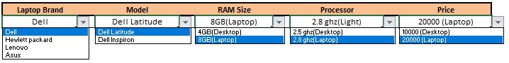
The final output after we repeat the process for fourth and fifth drop-downs, would look as shown in the below Figure.
Conclusion
Creating drop-down with array formulas is fun. I hope this article would help you in creating more sophisticated dashboards with multiple dependent dynamic drop-downs.
Check out our Tableau Pages
- Tableau Contractor San Francisco, CA
- Tableau Contractor San Jose, CA
- Tableau Contractor Los Angeles, CA
- Tableau Contractor San Diego, CA
- Tableau Contractor Sacramento, CA
- Tableau Contractor Dallas Fort Worth, TX
- Tableau Contractor Austin, TX
- Tableau Contractor San Antonio, TX
- Tableau Contractor Houston, TX
- Tableau Contractor Norwalk, CT
- Tableau Contractor Chicago, IL
- Tableau Contractor Atlanta, GA
- Tableau Contractor Philadelphia, PA
- Tableau Contractor Pittsburgh, PA
- Tableau Contractor Phoenix, AZ
- Tableau Contractor Boise, ID
- Tableau Contractor New York, NY
- Tableau Contractor Rochester, NY
- Tableau Contractor Jersey City, NJ
- Tableau Contractor Washington, DC
- Tableau Contractor Charlotte, NC
- Tableau Contractor Seattle, WA
- Tableau Contractor Miami, FL
- Tableau Contractor Boston, MA