Accessing multiple data sources using ADO and VBA in Excel

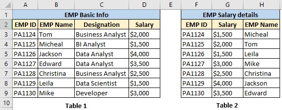
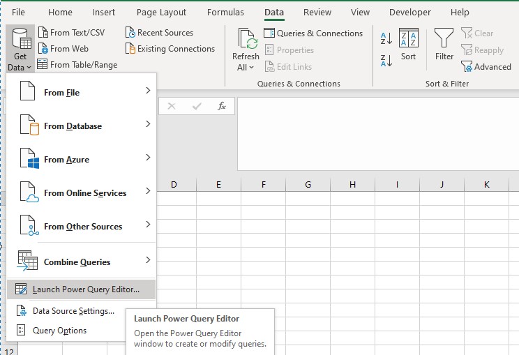
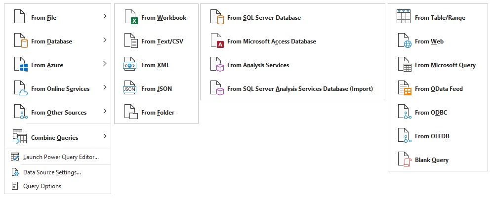
One way to load data into an Excel worksheet is to simply use “Get Data” option from Data tab. But it’s a manual process. In this article, let us look at another way to load data using VBA with ADO as the interface.

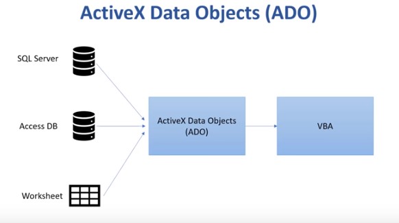
ADO stands for “ActiveX Data Objects”, the reason for using ADO in excel is that it acts as a common interface to get data from multiple sources. The main use of ADO is to unite all other data sources on to a single platform. If there was no ADO, then we would end up writing individual code for each data source.

ActiveX Data Object model to connect excel

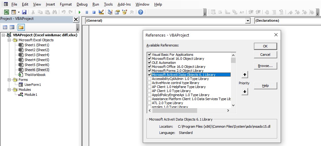
‘ADO’ is not a default object added into the Excel VBA library. So, we must add it by navigating as follows: Tools -> references -> Microsoft ActiveX Data Objects 6.1 Library. Look at the below image for reference.

ADO object 6.1 in excel VBA Library

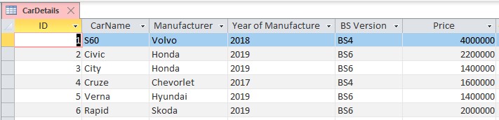
Let us write the VBA code using ADO object to load data from MS Access database. In this article we would be using “CarDetails” (MS Access Table) as the source DB table. Refer below snap to know more in detail.

Table in MS Access Database to connect to excel

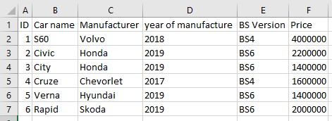
The below code will fetch the data from MS Access database and loads into the excel file. Let us look at the loaded data in the below image. You can customize the query and the source depending on the required data. Indeed, you can get data from any source using ADO interface without any glitch.

MS Access table copied to Excel using ADO and VBA

Step 1: First step is to declare the new ADO object as:
                   “New ADODB.Connection”
Step 2: Open the connection by providing the connection string. In this article let us consider MS Access connection string
            “Provider=Microsoft.ACE.OLEDB.12.0;”&”Data Source=”Location of the MS Access file;”
Step 3: Create a string object to write a SQL query
              Dim query As String
              query = “select * from CarDetails”
Step 4: Create a ‘New’ Recordset to open the connection and execute the query. Refer below code to get an idea
              Dim rs As New ADODB.Recordset
              rs.Open query,Conn
Step 5: Select the destination location to load the data. In this article, we have considered Excel as the destination file. So, select the specific range in the excel to populate the data
             Sheet1.Range(“A1:F1”).Value = Array(“ID”, “Car name”, “Manufacturer”,  “year of manufacture”, “BS Version”, “Price”)
             Sheet1.Range(“A2”).CopyFromRecordset rs
Step 6: Final step is to close the connection
              Conn.Close


Check out our Tableau Expertise Related Pages

MS Excel for Windows Vs Mac: Who wins the race?

Excel is one of the widely used spreadsheet applications created by Microsoft for Windows, MacOS, Android and iOS. In this article, we will be focusing on some of the major differences between Excel for Windows & Mac.

Power Pivot & Power Charts

The below table clearly shows the major differences in windows and MacOS versions of Excel.

Excel Windows and MAC differences

Static Charts can be depicted in Mac, but they are not interactive like Windows excel charts and they don’t update upon changing the source pivot table. Any pivot table having source data based on Excel data model will be unfilterable if the spreadsheet is opened by a Mac user. The following image shows an error message while opening a file in MacOS.

Pivot table error message in MacOS

VBA Editor User Interface

The VBA editor on Excel for Mac 2016 is in a sorry state compared to its windows counterpart.

  • ‘Properties’ window is missing
  • Developing a ‘User form’ in Excel for Mac by using design mode would be a tedious job compared to Excel for Windows

Importing VBA collections would be an added disadvantage

VBA Workbook and Worksheet events

If you are someone who uses worksheet events of VBA often, then you would be disappointed as there are no Workbook & Worksheet VBA events in Excel MacOS. Thus, you should rely completely on VBA modules only.

VBA Events in MAC pop error message

Default file location settings and Autosave workbooks

  • The windows version of excel enables you to set a default location for saving files. This setting is not available in Mac version of Excel
  • “AutoSave” is one of time saving features which automatically saves your workbook as a draft and enables you to retrieve older version of the file even if you didn’t save your changes. This feature too is no available in Mac version of Excel

Find and Replace formats

In windows, find and replace dialog has an option to find cells based on their formats (Say, background color) and it would replace the found cells of the same background. This is not available in Excel for Mac.

ActiveX Controls

ActiveX controls are intended to be used with VBA programming, but this feature is not available in Mac version of excel. Thus, Excel VBA pros are restricted to use Form controls in excel MacOS.

Relative references

Irrespective of operating system, relative references are very useful in creating dynamic range while recording macro. Windows allows user to record macros in both absolute and relative references, but Mac doesn’t have relative reference feature while recording the macro.


Check out our Tableau pages

XLOOKUP: A Brand-new formula in Office365

The wait is over!! Finally, Microsoft has released an update to Office365 with a brand-new formula “XLOOKUP”.

XLOOKUP has the following advantages, compared to its predecessors.

  • Can lookup on both left and right directions.
  • Exact match is default.
  • Can return FIRST or LAST match.
  • XLOOKUP also replaces VLOOKUP & HLOOKUP.

Earlier, INDEX-MATCH formula combination was used to lookup values where HLOOKUP & VLOOKUP fell short. Now, XLOOKUP can replace all other functions. It is a robust and easy to use formula which can lookup values from right to left and vice versa.

Syntax:

=XLOOKUP(lookup_value,lookup_array,return_array,[match_mode],[search_mode])

Explanation

Let us consider the below example to get deep insight of the formula. Our agenda is to fill column D of Table1 (Salary) using XLOOKUP

Two distinct tables for Xlookup

Lookup_value: Exactly same as VLOOKUP. In this scenario, let us consider Column B of Table1 as our lookup value.

Lookup_Array: Typically, the destination range/column where XLOOKUP will look for the match. Column H of Table2 would be our lookup array.

Return_Array: This argument is asking for the return value. In this case, we want salary column to be filled so we would consider Column G of Table2 as the return value.

[match_mode]: This is an optional argument in XLOOKUP formula. It can be any one of the following. By default, it is “Exact Match”.

  • 0 – Exact match
  • -1 – Exact match or next smaller item
  • 1 – Exact match or next larger item
  • 2 – Wildcard character match.

[Search_mode]: It can be either 1 or -1. “1” is to search from first to last and “-1” is from last to first.

Let us write the below formula in cell “D3” of table1 and the output looks as below.

XLOOKUP($B$3:$B$9,$H$3:$H$9,$G$3:$G$9,0,1)

Xlookup output

How to accelerate excel performance?

Efficiency is one of the key elements to evaluate any application. Excel has always topped the race in efficiency when compared to other spreadsheet applications. But there are some instances where Excel lags in performance which could affect productivity. In this article let us look at some of the key elements that would help to enhance the performance of Excel.

Excel Performance Accelerator

Excel 2007 and later versions have “Big grid” (1 Million rows and 16,000+ columns) compared to their previous versions. Since the capacity of the application has increased, there are more chances for performance degradation as we would be dealing with huge amount of data.

1. Switch to Manual Calculation mode from Automatic

By default, automatic calculation is the default option while working on Excel. In this mode, whenever we change the content of any cell in our workbook, all formula in all cells of all open workbooks would be recalculated. We won’t realize the time spent in formula recalculation as long as it is less than a tenth of a second, all put together. As this calculation time increases, annoyance starts to increase, especially for repetitive tasks. In this situation’s users can switch to “Manual calculation” option in the formulas tab. In this mode, formula would be recalculated only when ‘Calculate Now’ or ‘Calculate Sheet’ button is pressed.

2. Avoid Circular references

As calculations are single threaded, multiple references to one or more formula could slow down the performance. Minimizing the use of circular references can boost the formula calculation time.

Excel Circular reference

3. Avoid links across workbooks

Try to avoid links between workbooks. If links are not removed, opening of that workbook could end up in evaluating the link from the source. This can easily increase the calculation time. Best practice is to paste special the formulas into values, which can save your memory and increase calculation time as well.

4. Write efficient formulas

Writing efficient formulas will add value to the calculation time. Nested formulas, array formulas, unsorted columns, redundant data can lead to performance degradation. For example, VLOOKUP and HLOOKUP with exact match would take more calculation time than approximate match after sorting the same data. So, better understanding of logic and using the right formula can increase Excel performance.

5. Use conditional formatting cautiously

We should be very cautious while using any formatting option in Excel, especially while using conditional formatting because of its volatile nature. Apply the formatting only to the used range and make sure you haven’t selected the entire column/row while applying these formats. This can increase Excel performance.

There are many other elements to be considered to improve performance of an application. The above mentioned are few among them and these are the key to accelerate the performance of an Excel application.


Check out our Tableau pages

Intro to Power query in Excel

This tool is generally referred to as ‘Power Query’ when searching for information online. However, with Excel 2016, the tool is also commonly referred to as ‘Get and Transform’. It can link to external data from many different types of sources into local data model in Excel or display them as tables. It uses the M Language to record each step we make and lets us to modify those steps in way we want.

Power Query is one of the most powerful tools added to Excel. There is lot of potential to save time in repetitive data cleaning and formatting using this. It can be accessed by clicking Data -> Get Data -> Launch Power Query editor.

Excel get data option to select the data source

Connect, Transform, Combine and Share are the sequence of steps to blend data make the data model, using Power Query.

Phases of data transformation from data source in excel

Connect

Power Query can be connected to single or multiple data sources like Excel workbook, databases, feeds and cloud services. Microsoft always updates the new data connections to Power Query, so you should update the App to get them added.

Once you connect to any of the data sources then you can directly load data into excel or edit using Power Query by clicking on the option provided. The below snap shows the number of data connections available in Power Query.

Different data sources in excel

Transform

Power Query lets you remove column, change data type, merge tables etc. Each of these actions is a transformation. The above-mentioned options are available in Query Editor/Transform of the Power Query ribbon. The Query Editor records each step you apply to the data.

Transform option in Power query menu

Combine

You can combine data from multiple data sources into single data model to get unique view into the data. There is no specific option called combine in Power Query. You can achieve this by writing a query or merge/grouping different tables and make them a single table with a unique reference. We can load the merged data into excel for further analysis.

Share

After applying all the conditions/queries on the loaded data. The result will be the processed information. We can save, share or use it for further analysis. Typically, you can use these reports in excel, power BI or any other BI tools for analysis and visualization.