Conditional formatting is used to pick out important data from a huge list of data. Though it is a little difficult to use, knowing the basics can help us in whatever project we are working on.
We can use conditional formatting in many ways. Following are the two ways of using conditional formatting.
 Conditional Formatting in Same cell
 Conditional Formatting in Multi cell
 Conditional Formatting in Same cell
We can use this option, when we have to apply formats to the same cell. Let us take the example below to apply formats based on required conditions.
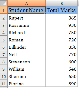
In column B of the above picture, the total marks of the students are displayed, we can identify the marks less than 700 and greater than 700 quickly by applying conditional formatting on column B.
Conditional formatting for the values Greater than 700.
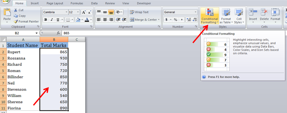
 Select the cells to format and select Conditional Formatting from Home menu.
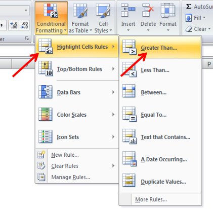
 Select Highlight Cells Rules and select Greater Than from the drop down.
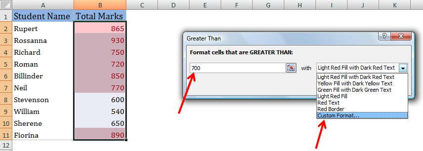
 Enter the number in the box provided for “Format cells that are GREATER THAN:”, and select ‘Custom Format’.
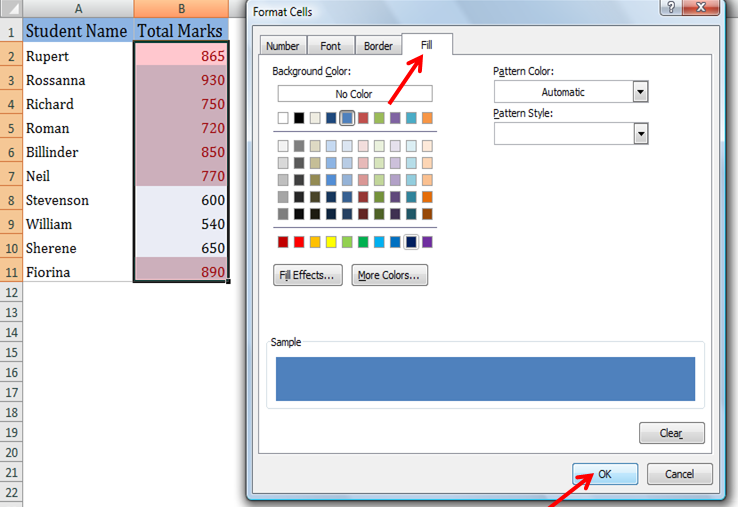
 Select Fill from Format Cells, Select a required color from Background color and select OK.
 The picture shows the result after applying Conditional Formatting.
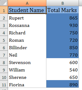
Conditional formatting for the values less than 700.
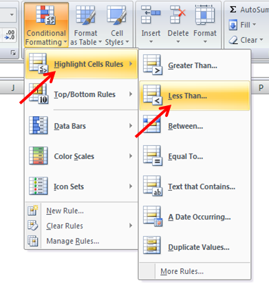
Select the cells which have to be formatted, select Conditional Formatting from Home menu, Select Highlight Cells Rules and select Less Than.
 Select the cells to format and select Conditional Formatting from Home menu.
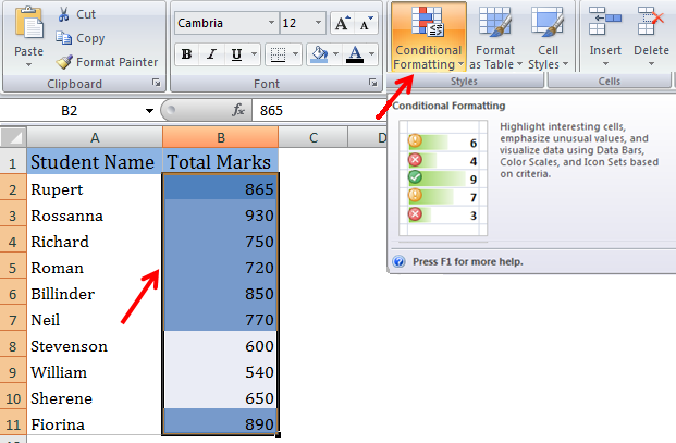
 Select Highlight Cells Rules and select Less Than from the drop down.
 Enter the number in the box provided for “Format cells that are LESS THAN:”, and select ‘Custom Format’.
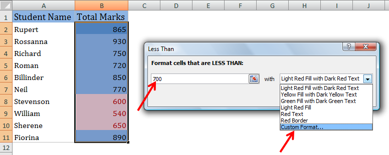
 Select Fill from Format Cells, Select a required color from Background color and select OK.
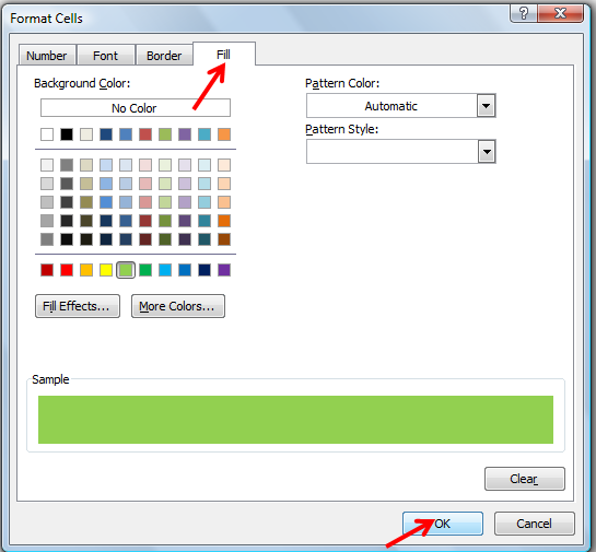
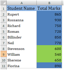
 The picture shows the result after applying Conditional Formatting.
 Conditional Formatting in Multi cell
This option is used
to apply formats to more than one cell based on one value. Let us take the example below to apply formats based on required conditions.
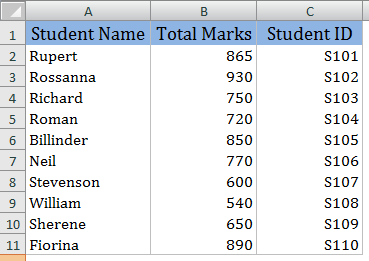
 Select the cells to format and select Conditional Formatting from Home menu.
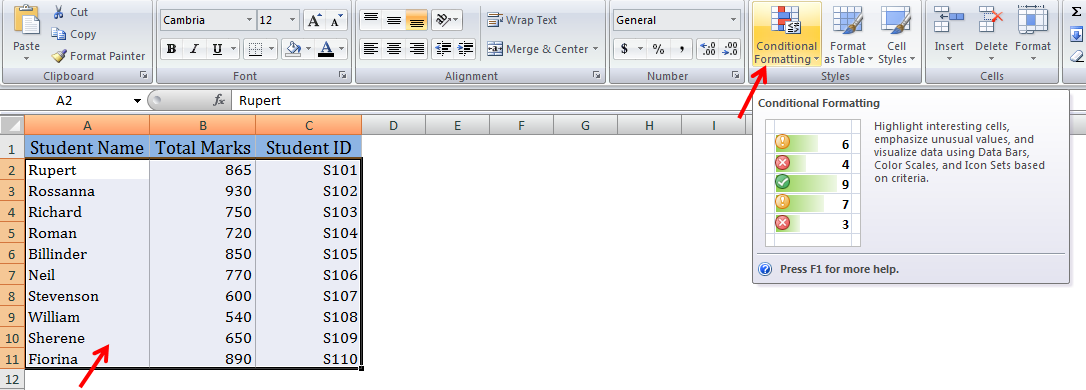
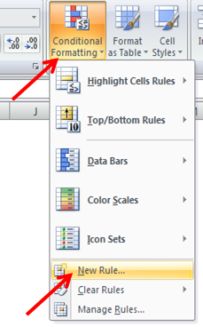
 Select
New Rule from the menu.
 Select Use a formula to determine which cells to format from New Formatting Rule window, enter the formula in the box provided for “Format values where this formula is true: , and select Format.

 Select Fill from Format Cells, Select a required color from Background color and select OK.

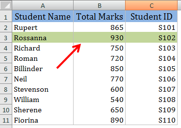
 The picture shows the result after applying Conditional Formatting.
————————————————————————————————————–
Vani is a Business Associate with p2w2, a Spreadsheet Solutions company. p2w2 has expertise in Excel Modeling, Excel Dashboards, Profitability Analysis, Excel Invoicesand Excel Bid sheets. You can contact us by email: cs [at] p2w2.com or call us at 305.600.0950.


Pretty! This has been an incredibly wonderful article.
Many thanks for supplying these details.